In the previous post we created 3 channels from the RGB original picture : Y’, Cb, and Cr.

We will now look that the luma histogram, so using the Y’ channel computed in previous post.

What is an histogram ?

It is a graphical representation of the pixel value distribution in a picture. It could be done by color channel in the RGB domain, it could also be done on the luma in the Y’CbCr domain.

We define some bins, for example 256, covering values from 0 to 255. It will be our X axis. Every histogram bin should contain the number of pixels with this value. It will be our Y axis.

For example, the bin 42 (so the 43rd bin, as we start at bin 0) will contain the number of pixels having luma=42.

What can we look in an histogram ?

To have a good contrast, a picture should use all the tones, from black to white. So the histogram should go from left to right. If contrast is poor, then most pixels will be in a limited histogram range. Let’s looks at some examples, done using gimp.

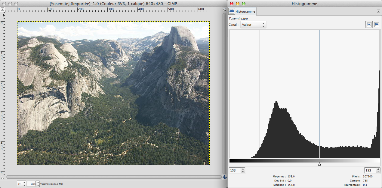
Original : contrast is OK

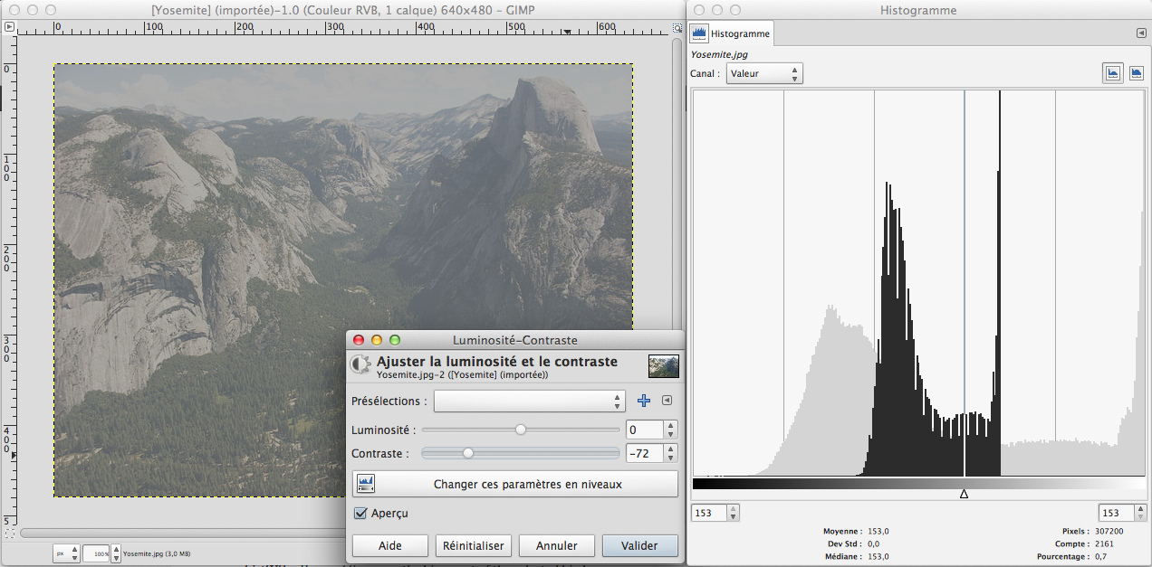
Low contrast : tones only in a limited histogram range

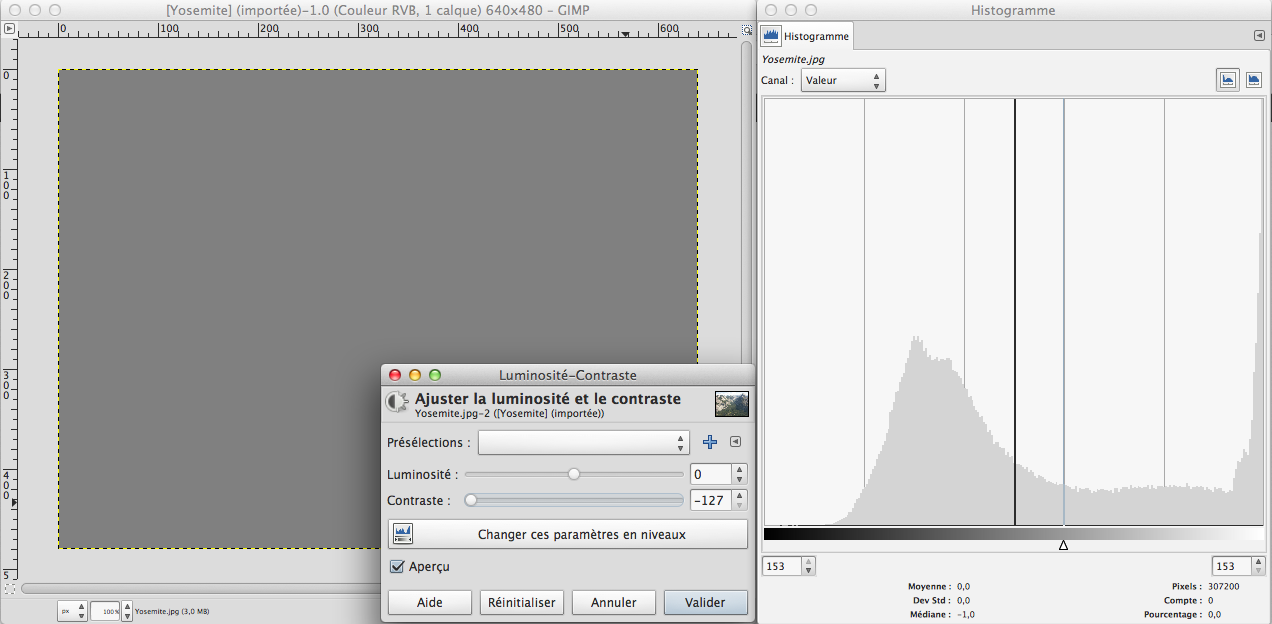
Extreme low contrast : all pixels are in one bin. It means the picture is ALL GRAY.

Getting the histogram from the Y’ channel

We will go through all the pixels, as usual. For every pixel, we will look the Y’ value. It will give us the histogram bin to update. This bin will just be incremented by one.

So in the code it will be :

// Loop through every pixel in the image, update histogram.
for (int y = 0; y < img.height; y++) {
for (int x = 0; x < img.width; x++) {
int loc = y*img.width + x; //computing 1D location of current pixel

hist[Y[loc]] +=1; //increase the bin count of the selected bin by 1.
}
}

Drawing the histogram

We will draw the histogram bin by bin. Every bin will be drawn as a vertical line. We will scale the bin relatively to the max value of the hist array.

for (int i = 0; i < 256; i++) {
int x,y;
x = img.width + i;
y = img.height;
line(x,y,x,y-(hist[i]*y/max(hist)));
}

Et voila !

You can check the result here. As always, there is a link to the full source code.

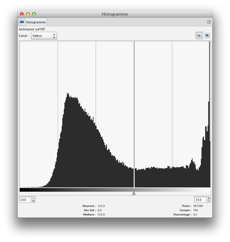
That’s all, we just did a luma histogram. Here is what Gimp is showing on the same picture after Y’CbCr decomposition, using ITU R470 256 option.

When looked at the same scale, the 2 histograms are very similar.